Gradients and Intercepts of Linear Functions

A Linear Function represents a constant rate of change. When plotted on a graph it will be a straight line.

A graph may be plotted from an equation $y = mx + c$ by plotting the intercept at $(0, c)$ , and then drawing the gradient $m$ , although it is normally easier to generate the points in a table and plot the graph.

The graph of a line can be used to find the equation by working out the gradient $frac(up)(along)$ which gives the $m$ value, while the intercept on the y-axis gives the $c$ value.

Example 1

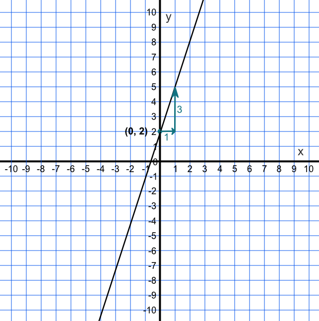
Draw a graph for the equation y = 3x + 2

Either plot a table for values of $x$ and $y$ or,

Using $y = mx + c$ :

$c$ is the intercept $y = 2$ when $x = 0$ and

$m$ is the gradient = 3 (3 up, 1 along)

Answer:

Graph plotted for y = 3x + 2

Example 2

Without drawing a graph, determine the coordinates for the intercepts on the $x-$ and $y-$ axes for $y = 4x - 4$ .

When $x = 0$ , then $y = 4 xx 0 - 4$ therefore $y = -4$ . Coordinate is (0, -4)

When $y = 0$ , then $0 =4x - 4$ therefore $x$ = 1. Coordinate is (1, 0)

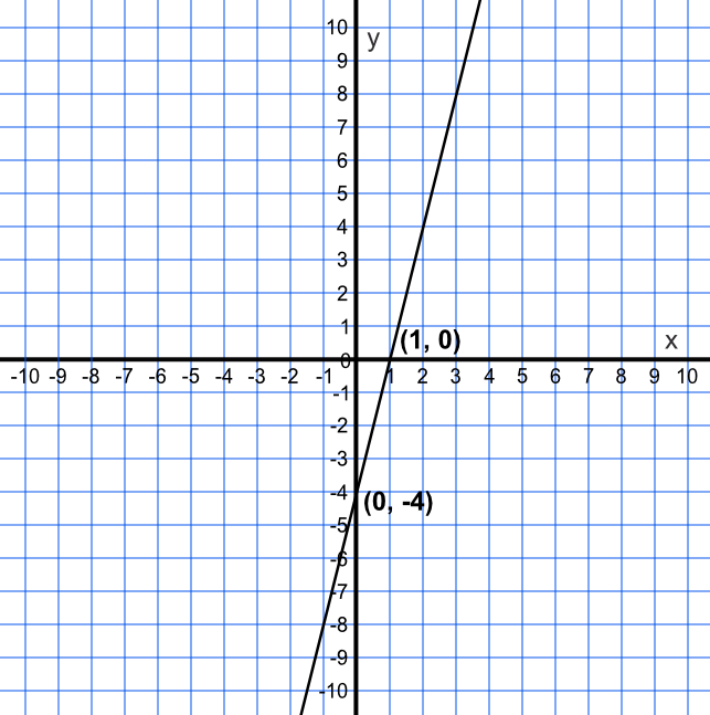
Plot of graph when finding intercepts for y = 4x - 4

Answer: (0, -4) and (4, 0)